
The phrase "autonomous ERP" gets used loosely in the JDE space, and the looseness hides a real engineering question. What does it actually take to let a JD Edwards integration make a decision and act on it without a human approval step? Not in the abstract — in the math. Because the difference between an integration that recommends and an integration that decides is a numerical threshold, a defined feature vector, and a set of bounded-risk operations that can be reversed if the decision was wrong. JD Edwards Integration: the math behind autonomous ERP is a phrase that resolves to a small set of formulas, a clear architecture, and a much larger set of organisational decisions about which actions deserve which level of trust.
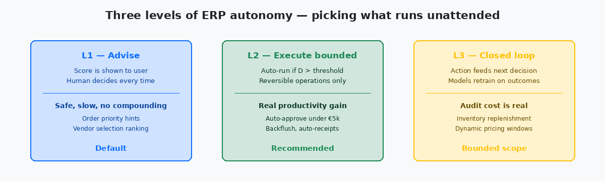
Most of what gets shipped as "AI-powered ERP" today sits at the lowest tier of autonomy — a model produces a score, the score is shown to a human, the human clicks Approve. That is useful, but it is not autonomy. Real autonomy means the score crosses a threshold, the action fires, and a control loop catches the wrong answers fast enough to keep the financial damage bounded. The math that holds this together is older than any current product wave, and worth writing down explicitly before the next vendor pitch.
The decision score: what the formula actually contains
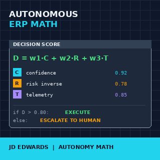
At the heart of every autonomous action sits a scalar decision score, computed from a small set of inputs and compared against a threshold. The general form is a weighted sum: D equals w1 times C plus w2 times R plus w3 times T, where C is the model's confidence in its recommendation, R is the inverse of the estimated risk (so high R means low risk), and T is the agreement of the runtime telemetry with the assumed business state. The weights w1, w2, w3 sum to 1 and reflect how much the organisation trusts each signal.
The threshold is the only number the business owner needs to set explicitly. Below the threshold the action does not fire and the recommendation is passed to a human. Above the threshold the action fires automatically. Setting the threshold at 0.95 produces something close to advisory behaviour; setting it at 0.70 produces aggressive autonomy with frequent corrections. Most production deployments I have seen sit between 0.80 and 0.88 — high enough that errors are rare, low enough that the automation actually saves the work it was built to save.
The confidence input C comes from whatever model is producing the recommendation. A logistic regression scoring an invoice match returns a probability directly; a more complex model exposes a calibrated confidence through standard techniques. The risk inverse R is the part that ERP teams routinely underbuild — it should capture not just the financial magnitude of the action but also its reversibility. Posting a 50,000 EUR journal that cannot be unposted without a manual reversal carries different R than authorising a 50,000 EUR purchase order that can be cancelled before it ships.
The telemetry term T is what stops the system from acting on stale or contradicted signals. If the recommendation assumes that F4111Item Ledger File — the JDE table that records every inventory transaction. Its current state is the ground truth for what is actually on hand at any moment. shows 300 units on hand and the latest cycle count says 50, T collapses and the threshold is not crossed. The autonomy is not "we trust the model"; the autonomy is "we trust the model when reality agrees with the model's assumptions". The distinction is what separates working autonomy from expensive incidents.
What "reversible" actually means inside JDE
The first design decision in any autonomous JDE integration is which actions are reversible enough to delegate. The intuitive answer is "everything is reversible eventually", which is true and useless. The operational definition that matters is whether the reversal can be performed inside a short window without a manual audit trail and without touching downstream systems that have already consumed the action.
Purchase order creation is reversible by cancellation, cheaply, before the supplier confirms. Once the supplier confirms, reversibility drops sharply because external commitments now exist. Sales order creation is reversible by line cancellation right up until shipment confirmation; afterwards the reversal involves returns processing. Inventory adjustments are reversible by reverse adjustments, but they leave a permanent audit trail in F4111 — reversible in effect, not in record.
Journal entries are the boundary case where most teams stop. A posted journal can be reversed, but the reversal is a new transaction with its own date, its own number, its own audit trail. For period-close reasons and for auditor reasons, very few organisations want autonomy to operate freely against F0911. The pattern that works is autonomy on the staging side — autonomous creation of pre-posting batches in F0911Z1, with the actual post still requiring a daily human review.
The classification is not absolute; it is per-installation and per-business-process. The math above does not care which actions you decide are reversible — it cares that the R term encodes the answer correctly. An action your business treats as reversible gets a high R and crosses the threshold easily; an action your business treats as irreversible gets a low R and effectively never crosses the threshold without a human in the loop.
Feature construction: turning JDE state into a vector
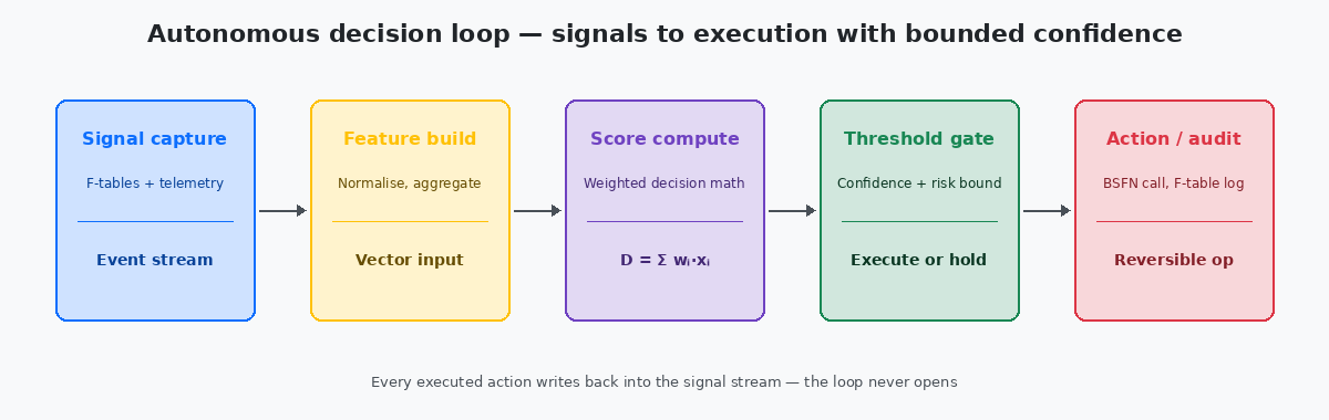
The decision score depends on features, and features depend on what the integration can read from JDE in time to compute them. The mechanical work that makes autonomous ERP feasible is feature construction — turning the relational state of JDE tables into a small fixed-size numerical vector the model can consume.
For an autonomous invoice-matching decision, the feature vector typically contains 20 to 40 fields: the invoice amount, the matched PO amount, the difference normalised by PO amount, the receipt quantity, the receipt date, the supplier's historical match accuracy from the last 200 invoices, the supplier's open-balance with the company, the buyer's typical tolerance for this commodity class, the time of month relative to period close, and several derived ratios. Each of these comes from a specific F-table read with a specific filter, and the latency of those reads is what determines whether the integration can decide in the few seconds before the human queue would have picked it up.
The feature build step is also where the telemetry signal T is computed. The model assumed a receipt existed; T confirms the receipt is in F43121 with the expected quantity and date. The model assumed the supplier was not on hold; T checks F0401 for the hold flag. Mismatches between assumption and reality become input to the score, not silent failures. This is mechanically tedious and has to be re-implemented for every business process the autonomy covers — there is no shortcut, and a vendor pitch that does not explain the per-process feature work is a vendor pitch that has not done the work.
The right place for the feature-build code is a custom BSFNBusiness Function in JDE — compiled C or NER code that encapsulates reusable business logic. The natural home for feature extraction because it can read multiple F-tables in one server-side call. per business process, called from an Orchestration that delivers the vector to the model. Server-side feature extraction is fast (single-digit milliseconds per call when the indexes support it), keeps the database reads inside JDE's connection pool, and makes the feature definitions versionable through OMW like any other custom code.
Calibration: why the threshold cannot just be set to 0.85 and forgotten
A threshold value is only meaningful if the score distribution behind it is calibrated. A model that returns 0.85 for cases where it is actually right 60% of the time and 0.90 for cases where it is right 95% of the time has a non-monotonic score, and any fixed threshold against that score behaves randomly in practice. Calibration is the discipline that makes the threshold meaningful, and it is the part of the math most ERP deployments skip.
The standard calibration check is a reliability diagram: take the last few thousand decisions, bin them by predicted score (0.70 to 0.75, 0.75 to 0.80, and so on), and for each bin compute the empirical accuracy. A well-calibrated score returns 0.85 for cases that turn out right 85% of the time. A score that returns 0.85 for cases right 70% of the time is overconfident in the high bins and needs to be recalibrated, typically through Platt scaling or isotonic regression applied as a post-processing step.
The recalibration cadence depends on how fast the underlying business changes. A new product line added to the catalogue, a major supplier change, a price renegotiation that shifts the distribution of invoice values — any of these can decalibrate the score within weeks. The discipline that holds the system together is automated reliability checking on a fixed cadence (weekly is typical) with an alert when calibration drifts past a defined tolerance.
The same calibration framework drives the threshold setting itself. The business owner does not set 0.85 by intuition; the business owner sets the maximum acceptable error rate (for example, 5% wrong autonomous decisions across the targeted action class), and the threshold that delivers that error rate is read off the reliability curve. This is the engineering move that turns "set a threshold" from a guess into a defensible specification.
The control loop: what catches the wrong answers fast enough to matter
Even a perfectly calibrated score will be wrong some of the time, and the autonomy is only safe if the wrong answers are caught and corrected before they compound. The math is incomplete without a defined control loop that monitors outcomes and feeds back into the decision system.
The control loop has three components: an outcome signal that records what actually happened after each autonomous action, a comparator that flags outcomes inconsistent with the predicted state, and a circuit breaker that can suspend autonomous action when the inconsistency rate crosses a defined level. For an autonomous invoice match, the outcome signal is the eventual payment reconciliation; the comparator flags matches that were later disputed or reversed; the circuit breaker pauses autonomous matching for a process or supplier when the dispute rate in the last 200 actions exceeds a percentage agreed with the business owner.
The circuit breaker is the part most ERP integrations under-implement, because it is the part that has to fail safely under organisational pressure. A pause in autonomous matching during the busiest payment week of the month creates friction with the AP team, and the temptation is to override the breaker manually. The math does not care about that temptation; the math says the breaker exists to bound the cumulative error, and an integration where the breaker can be silently disabled has lost the property that distinguished it from a naive automation.
The feedback step is what closes the loop in the genuine sense. Outcomes flow back into the training data; the model retrains on the corrected ground truth; the calibration recomputes against the new distribution. None of this is mysterious — it is the standard machine learning operations stack adapted to the latency and audit requirements of an ERP. The adaptation is the engineering work; the math is the framework that makes the adaptation principled instead of ad-hoc.
For more on this side of JDE work, the related articles on Orchestrator design patterns, on JDE telemetry pipelines, and on F-table integration architecture cover the surrounding technical layer. The technical project portfolio on this site documents two production autonomous-integration deployments where the math described above moved from whiteboard to running code.
