The hardest question to answer on any mature JDE installation is one of the simplest to ask: "if I change this table, what custom application breaks?" Mapping business view dependencies in JD Edwards EnterpriseOne custom applications is the discipline that turns that question from a multi-day forensic exercise into a query that returns in seconds. Most installations have between 80 and 400 custom business views layered on top of standard and custom tables, called by an unknown number of applications, UBEs and forms — and nobody has a current picture of which depends on which.

The cost of not knowing is paid every time something changes. A column added to F4211. A new index on F0911. A custom table renamed during a clean-up. Each change ripples through whatever business views reference the affected object, and every BV affects every application built on top of it. Without a map, the impact is discovered when something breaks in PY, or worse, in PD.

Why business views are the right place to anchor the map

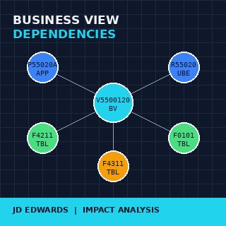
A business view in JDE is not a database view. It is a metadata object that selects columns from one or more tables, defines joins between them, and exposes the result as a single rectangular dataset that forms, applications and UBEs bind to. The BV sits between the tables and the code, which is exactly why it is the right node to use as the anchor of any dependency map.

Anchoring on tables alone produces noise — every application reads tables, directly or indirectly, and the resulting graph is too dense to be useful. Anchoring on applications produces gaps — applications call BVs that join across multiple tables, and a table-level question routed through an application-only map loses fidelity. The BV is the natural join point: it knows which tables it touches and it is known by every caller above it.

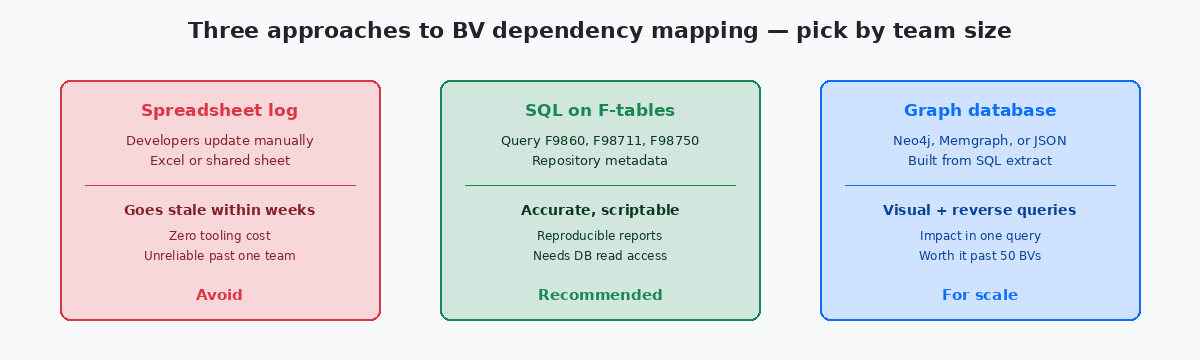
On the upstream side, every BV declares its source tables in the spec, recorded in the F98711Business View columns metadata table — the JDE repository table that records which columns of which tables each business view exposes, along with join definitions. repository table. On the downstream side, every form, application and UBE that uses a BV records the relationship in F9860 with a source type that identifies the consumer. Two SQL queries, properly joined, produce the complete graph for the entire installation.

The other reason to anchor on BVs is that they change less frequently than the code that uses them. A BV with twenty consumers might be modified once a year; the twenty applications above it might be touched twenty times in the same period. A map built on the stable layer holds its accuracy longer between regeneration cycles.

The repository tables that hold the truth

The JDE repository — the metadata about every object in the installation — lives in a small set of system tables that are read-only from the developer's perspective and consistently underused for analysis. The four that matter for dependency mapping are F9860, F98711, F98712, and F98750.

F9860 is the object librarian master. Every BSFN, application, UBE, business view, and table has a row here, with OBNM (object name), FUNO (function use, identifying type) and SRCTYPE (source type, distinguishing BV from APPL from UBE from TBL). A simple query against F9860 filtered to FUNO values for business views returns the complete list of BVs in the installation; filtered to applications, the complete list of forms above them. The filter values are documented in the standard table definitions and they do not change between Tools Releases.

F98711 is the column-level join table for business views. Every column a BV exposes is a row, with the source table and the source field. Aggregating F98711 by BV name gives the complete table-level footprint of each view — which is exactly what the upstream side of the dependency map needs.

F98712 records form and report sections that bind to a BV. A custom application that calls three different BVs across its forms produces three rows in F98712 keyed by the application name and the BV name. This is the downstream side: which callers use which views.

F98750 is the spec data store on modern Tools Releases — the binary spec content is stored here, indexed by object. For dependency mapping, F98750 is usually not the primary source because the readable metadata is already in the other three tables; F98750 becomes relevant only when chasing spec-level details that the metadata tables flatten away.

Building the graph: from SQL extract to navigable structure

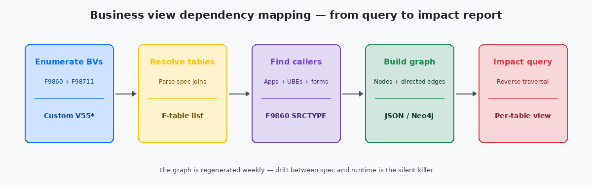
The mechanical part of the mapping is straightforward and routinely overcomplicated. Three SQL queries against the repository, run in sequence, produce everything needed for a complete dependency graph for an installation of any size.

The first query enumerates every custom business view — filtered by name prefix, typically V55 through V59 on shops that follow Oracle's reserved namespace convention. The output is a flat list with BV name, BV description, and last-modified timestamp. On a typical mid-sized installation this returns 80 to 300 rows in under a second.

The second query resolves each BV to its source tables. Joining F9860 to F98711 by OBNM and grouping by the BV plus the source table name produces a many-to-one list — one row per BV-to-table relationship. A BV that joins F4211 and F4101 produces two rows. A BV that touches eight tables produces eight. The total volume here on a real installation is typically 200 to 1,500 rows.

The third query finds every caller for each BV by reading F98712 and joining back to F9860 to enrich the caller with its type and description. This is the largest of the three outputs because a popular BV may have twenty or thirty callers; total row counts here run into the thousands on larger installations, but still trivial volumes for any modern database.

The three result sets become the edges of a directed graph: tables point upward into BVs, BVs point upward into callers. Stored as JSON, the graph fits in a few hundred kilobytes and can be loaded into any visualisation tool from Neo4jA graph database widely used for dependency, network, and relationship analysis. Stores nodes and directed edges natively and answers reachability queries with single Cypher statements. down to a static HTML page with a force-directed layout library. The visualisation matters less than the underlying structure — the same JSON answers programmatic queries just as well as visual ones.

The impact queries that justify the effort

A dependency graph that is never queried is documentation theatre. The queries that justify building it are the ones that answer real questions developers and CNC teams ask under pressure.

The first impact query is reverse traversal from a table: given that F4211 will gain a column next sprint, list every custom BV that selects from it, and for each BV list every caller. The answer drives the regression test plan. On a graph with 200 BVs and 2,000 callers, this query returns in tens of milliseconds and produces a list that is exhaustive in a way no spreadsheet ever was.

The second impact query is forward traversal from an application: given that the custom P55020A is about to be deprecated, list every BV it uses, and for each BV check whether any other caller depends on it. Views with no other consumer become deprecation candidates themselves, and the chain continues down to tables that nothing else reads. This is the query that drives technical debt cleanup — the candidates surface themselves once the graph exists.

The third query is orphan detection. Custom BVs in F9860 that have zero rows in F98712 are orphans — they exist in the repository but nothing calls them. Custom tables that no BV selects from are deeper orphans. On a 20-year-old installation, orphan counts typically run from 5% to 15% of the custom estate, and every orphan is dead code that still has to be carried through every upgrade. Surfacing them is the first practical use of the graph on most installations.

Keeping the map honest: regeneration cadence and drift

The single failure mode of any dependency map is staleness. A graph generated once at the start of a project and never refreshed is wrong within weeks — every check-in to OMW that adds or modifies a BV creates a delta the static graph does not know about. The discipline that keeps the map honest is automated regeneration on a schedule the team actually follows.

The cadence that works on most installations is weekly. A scheduled job — a shell script, a small UBE, or a Python script connected to the JDE database — runs the three repository queries, builds the JSON, archives the previous version, and publishes the new graph to whatever location the team uses. Weekly is frequent enough that the map is never more than a few days behind reality, and infrequent enough that the job is not noisy.

The diff between consecutive snapshots is more useful than any single snapshot. New BVs that appeared this week, BVs whose source tables changed, BVs that gained or lost callers — these are the items worth surfacing in a team's weekly review. A BV that suddenly grew a fifth table in its join is a code review opportunity; a BV that lost its only remaining caller is a deletion candidate. The diff is twenty lines of script and it converts the graph from a reference document into a feedback loop on what the team is actually building.

For more on the surrounding territory, the related articles on retrofitting copies of standard, on Tools Release upgrade scoping, and on F-table archival strategies cover the operational layer this map sits on. The technical project portfolio on this site documents two production dependency tools that produced the patterns described here.